10 Essential SEO Excel Hacks to Increase Productivity

SEO is evolving continuously and requires in-depth analysis of data to track results, evaluate the performance of a campaign, create marketing strategies, etc. So, it is very important to manage this huge amount of data and information to carry on a campaign in an organised and effective manner. Excel plays a very important role in making this task easier and helps to manage complex data to create reports, conduct audits, and analyse data.

In this article, we will discuss Ten SEO excel tips and formulas that will help in SEO tasks and increase productivity.

Extract Domain Name from URLs

Formula:

=LEFT(url,FIND(“/”,url,9))

In SEO you would often come across task where you may need to extract domain names from the list of URL dump you got from an audit tool. In the above formula url if you wish to extract the domain name from the url the above generic formula will work wonders.

Example:

=LEFT(A2,FIND(“/”,A2,9))

A2 contains your url – https://www.dietseo.com/technical-seo/

Starting from left the Find function looks for “/” character in the URL starting at the 9th character https://. The FIND function will return the 3rd instance of “/”(the first time after the double slash in the protocol). In our case, the FIND locates the third instance of “/” at the 15th character in the URL. This is how the domain is extracted using the above formula.

Wild Cards

There are 3 different wildcards which have different applications in Excel: ‘’, ‘?’, ‘~’. The asterisk () can take place of any number of characters, Question Mark (?) takes the place of a single character and Tilde (~)tells Excel that the following character should be treated as a normal character and not a wildcard.

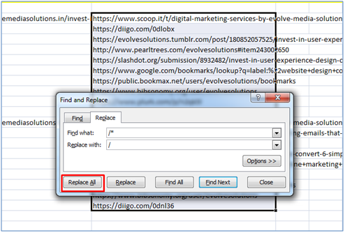
For example, if you have a long list of links but you only want to keep one sample URL from each domain in the sheet. Then, you can reduce every single URL to only its top-level domain by finding and replacing for /* – the star is a wildcard that removes everything after the first backslash.

Text to Column

This feature can be used in SEO to separate subfolders or divide up subdomains and root domains.

Using a delimiter “/” you can split the URL into various columns.

Find and Replace

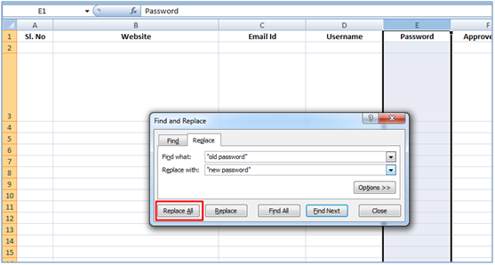
This feature helps to search any common data or text in the sheet and replace it with the desired text. For example, if you want to replace the same old passwords of a list of websites with the new one, then this feature can be used.

Select the whole column where you want to replace data and then use the shortcut ‘Ctrl + H’ to bring up the ‘Find and Replace’ dialog box.

Remove Hyperlink

Excel identifies text starting with http:// or https:// as a hyperlink by default and you can see the text in blue font colour and underlined. Every now and then the links get clicked and open in your default browser. To avoid this, convert them into regular text to make the task easier.

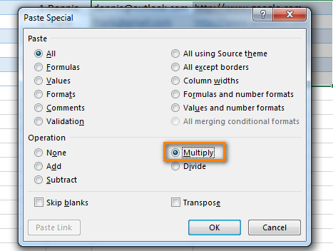
All the hyperlinks can be converted to text by using the shortcut ‘Ctrl + A’ twice to select all the cells in the sheet. Then right-click any cell and click ‘Remove hyperlinks’ OR Select entire column then Paste Special and select multiply. This way you can remove hyperlinks in bulk.

Formatting with ‘Proper’

Reformatting data in a proper case can be very time consuming if done one by one. Most of the times, if the keywords or some text is in lower case and you want them to be in the capitalised format, then this formula can help.

Create a new column for capitalised text, and insert the formula as shown in the image.

Formula:

=PROPER(Text)

CONCATENATE Function

CONCATENATE function purpose is to join text items together and returns the result as text.

Example:

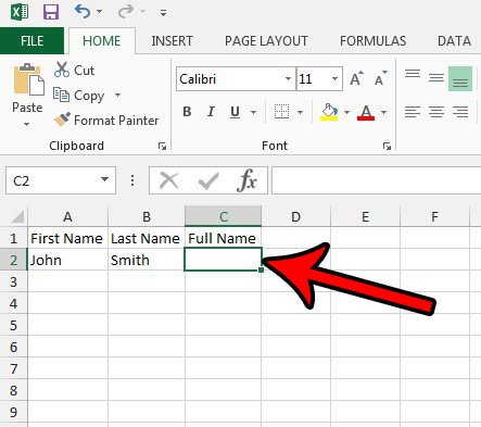
=CONCATENATE(A2,” and “,B2) // returns “John and Smith”

In the example shown, the following formula returns the string “John and Smith”:

VLOOKUP

To search from a large amount of data from a spreadsheet is very difficult and this is where VLookUp comes to your rescue. For a specified value, the VLookUp function finds it in one column of data and returns the corresponding value from another column.

The formula displayed in the image looks for a value in the left column of a table, and then gives you the value in the row from a column you want.

• Lookup_value: this is what you are searching.
• Table_array: this is where you want to search for it.
• Col_index_num: this is what you want the formula to return.
• Range_lookup: if you want an exact match, mark this is FALSE.

VLOOKUP only works if the data you need is in the first column (the left-most column) and the data is in ascending order (A-Z).

This is the most used function in excel for SEO’s especially if you are tracking exhaustive list keywords every month.

LEN – To Calculate the Length of URL, Title, Description

This feature helps to easily calculate the number of characters in a title, description, or any text.

Formula: =LEN(Text)

TRIM – To Remove Extraneous Spaces

Some times you might end up wonder why some of my excel formula’s aren’t applying correctly. This could be due to some extra spaces within the cell. This function helps to properly format a large amount of data with extra spaces. It easily removes the extra spaces but keeps the required spaces between words.

Formula: =TRIM(Text)

Conclusion

These SEO excel tips, tricks, and formulas make it easier to work with a large amount of data and information and make the SEO process more effective. Learning these hacks will help you to keep the data sorted and organised.